1.Introduction
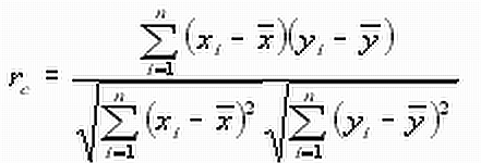
If the rate of
correlation between the data sets xi and yi
is to be
determined (in both cases i=1, 2, …, n), in the classical
mathematical
statistics (see e.g. Cramér 1945) the application of the
following formula is
proposed:
 (1)
(1)
(x and y are the mean values
of the data xi and
yi ,
respectively; the
index c
indicates that rc is
a calculated
value of the correlation coefficient and not the true
rt value
of it). For Gaussian distributions in Cramér 1945 also the
analytical formula
of the probability density function of rc is
given for the values of
rt and n. This formula is
cited as Eq. 2. in Steiner and
Hajagos 2008, too. For some cases even the f(rc)
curves are shown in
Cramér 1945; a such figure is cited in
Steiner 1990 on page 265 for n=10. The curves show really great degree
of
uncertainty if there are few data-pairs for the calculation of rc
,
the authors of the present article, however, mention self-critically
that in
the paragraph ofter Eq. 3. in Steiner and Hajagos 2008 the consequence
is too
pejoratively ( and too categorically) formulated: the value n=10 is
only for
our actual theoretical treatments unacceptable small. The formulation,
otherwise, in such degree of generality cannot be valid: the expert has
in some
cases not more data pairs as ten.
2. The concepts of robustness and
resistance
Before some decades two new concepts appear in the modern statistics: robustness and resistance (see e.g. Huber 1981).Robust is the statistical method if it is applicable with great enough statistical efficiency for a not too short interval of probability distribution types: the practitioner needs that the method must be applicable for all types which can occur in his discipline. As in the geosciences even the Cauchy-type can occur and Tarantola 1987 proposes the use of such statistical algorithms which are able to handle also the Cauchy-type even if not this distribution is characteristic to the actual problem but it can be justifiably suspected that outliers can occur in a not negligible percent therefore our statistical methods must be applicable also for data which are distributed according to the Cauchy-type.
In the paper Steiner and Hajagos 2008 is shown that Eq.1. cannot be applicated if the xi and yi data are Cauchy-distributed, consequently this formula for the calculation of the correlation coefficient is not robust.
The goal of the present article
is, however, to investigate
the resistance of Eq.1. , i.e.,the resistance of the classical
correlation
coefficient. Resistant against outliers is the statistical algorithm if
the
result is not (or not significantly) influenced by outliers, i.e., by
such data
wich
are of unknown origin:
strange in the sense that they do not belong to the regular data set.
Immense
causes can originate outliers (trivial examples are the erroneously
typed data)
and if the resistance is theoretically investigated the artificial
outliers are
not seldom very far from the regular data set. E.g., Andrews 1972 by investigating the
so-called
breakdown bounds of different estimates of location used the following
100
data: 100-J data are generated according to the
standard Gaussian probability density
function  and the outliers are
100; 200; …; j*100; …J*100. This means that
outliers can have values of some
thousands, too, although the standard Gaussian data are well known in
the
(-3;+3) interval („3s
rule”).
and the outliers are
100; 200; …; j*100; …J*100. This means that
outliers can have values of some
thousands, too, although the standard Gaussian data are well known in
the
(-3;+3) interval („3s
rule”).
On page 184 in the book Steiner (ed) 1997 the figure shows that the most frequent value denoted by M (as estimate of location) using k=2 tolerates even J=10 such outliers: till this limit the M-value is less than 0.02 (instead of the true value zero). The calculation method of the most frequent value as a statistical algorithm can be called justifiably as resistant.
3. Distortion
of
the classical correlation coefficient caused by outliers.
Let be assumed the simplest case: the xi and yi data are equally standard Gauss-distributed, i.e., the are generated according to the density distribution
respectively;
the
xi and
yi data
are uncorrelated (i.e.,
the true value of the correlation
coefficient equals zero: rt =0).
If 99 (xi , yi) data-pairs are according to the foregoings generated, they define 99 points inside the circle on Fig.1. The distortions of the rc-values (see Eq.1.) caused by one single outlier (only 1% of the data-pairs) were investigared if this outlier is near or far from the circle of the regular points. On Fig.1 the simple „menu” of outliers is given by points with series number; the x=y outliers are the followings: 1:(3;3); 2:(4;4); …; 18:(20;20).
For outlier-free case the f(rc)- curve is given for 100 Gaussian distributed points inside the circle on Fig.1 in Steiner and Hajagos 2008. The half-value width of this curve is greater than 0.2 ; consequently, Monte-Carlo calculations are needed to each outlier to have that distorted rc-value which can be accepted as the most probable one. In the justcited article only ten result was given for only one outlier (which corresponds to the (10;10) in our actual menu). These values bring about 0.5 – insted of zero –demonstrated that the classical correlation coefficient is not resistant. This justification of the existence of irresistance was enough as the main goal of this article was to present resistant alternatives for the calculation of the correlation coefficient (see Eq.8) and to investigate these new resistant characteristics.
In the present paper the regularity of the distortions caused by the outliers shown in Fig.1 are to be determined accurately enough, therefore for each outlier, 101 times were 99 Gaussian points generated, 101 rc-values were calculated according to Eq.1 and the median of these rc-values were determined; this procedure was 5 times repeated and finally the median of the 5 medians were accepted as a properly accurate result. These rc-values are represented in Fig.2 for each outlier defined in Fig.1. The distortion equals 0.2 even if the outlier is not too far: ( see e.g. the case of the (5;5) outlier series number 3) which is half so far from the origin as the above mentioned (10;10) outlier (remember that in Steiner and Hajagos 2008 the distorting effect of this was shown in Fig.1).
4. A
short not to the meaning of the word „outlier”
The expression „outlier” has pejorative meaning if we have to characterize the whole set of data ( or the whole of pairs of data as in the above discussed cases): we have seen that the result can be even misleading in presence of a single outlier. The outliers are, however, not always „wrong” data (e.g., they were erroneously typed); in the contrary, in som discipline of science they contain the most valuable informations. In the following paper of J. Verő 2008 fortunately there are given also concrete examples of such type. Consequently, there is given every reason to hope that in this way the reader is correctly informed about the Janus-faced character of the outliers.
A last remark: in some cases the most frequent value M and the dihesion e of the xi data (i=1, 2, …, n ) are able to characterize the value of information of the outlier (denoted by V(xj)) if the letter can be accepted approximately proportional to the distance between the valuable outlier and the dense lying set of points:
nbsp;  (2)
(2)
The expert of the discipline
decides if this way to the
selection and valuation of the far lying
data is convenient for him or n
value-pairs of two independent standard Gaussian distributions. Consequently the
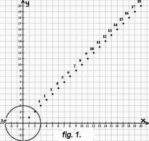
points marked with serial numbers are in this case outliers. ( Near the origin two
„inliers” are also given without series numbers.)
Fig. 2. The most probable rc-values calculated according to the classical formula of the
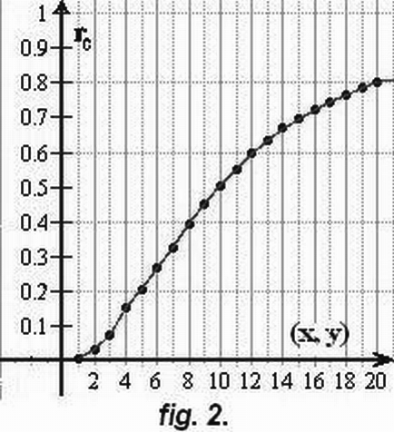
correlation coefficient (see Eq. 1.) if 99 value-pairs are generated according to the
standard Gaussian rule ( see the circle on Fig. 1.) and only a single outlying point is
taken into consideration ( characterised by the same value of x and y, see Fig. 1.). The
Fig. 1. in Hajagos and Steiner 2008 corresponds to the case x=y=10 resulting in the rc-
Value of 0.5 but even if the outlier is half so far, i.e., x=y=5, rc=0.2 holds instead of zero.
References
Andrews, D.
F.,Bickel, P. J., Hampel, F. R., Huber, P. J.,
Rogers, W. H., Tukey, J. W. 1972:
Robust Estimates of Location. Survey and Advances.
Princeton University
Press, Princeton, New Jersey, 373 p.
.Cramér, H. 1945: Mathematical Methods of Statistics.
Almquist & Wiksells, Uppsala, 575 p.
Huber, P. J. 1981: Robust Statistics. Wiley, NewYork, 308 p.
Tarantola, A. 1987: Inverse Problem Theory. Elsevier,
Amsterdam, 613 p
Steiner, F. 1990: Introduction to Geostatistics ( in
Hungarian).
Tankönyvkiadó, Budapest, 357 p.
Steiner, F. (ed.) 1997: Optimum Methods in Statistics.
Akadémiai Kiadó, Budapest, 370
p.
Steiner, F., Hajagos, B. 2008: Different characteristics of
the correlation of two sets of data
( in Hungarian). Magyar Geofizika.